CatBoost Enables Fast Gradient Boosting on Decision Trees Using GPUs
Machine Learning techniques are widely used today for many different tasks. Different types of data require different methods. Yandex relies on Gradient Boosting to power many of our market-leading products and services including search, music streaming, ride-hailing, self-driving cars, weather prediction, machine translation, and our intelligent assistant among others.
Gradient boosting on decision trees is a form of machine learning that works by progressively training more complex models to maximize the accuracy of predictions. Gradient boosting is particularly useful for predictive models that analyze ordered (continuous) data and categorical data. Credit score prediction which contains numerical features (age and salary) and categorical features (occupation) is one such example.
Gradient boosting benefits from training on huge datasets. In addition, the technique is efficiently accelerated using GPUs. A large part of the production models at Yandex are trained on GPUs so we wanted to share more insights on our expertise in this area.
Let’s look more closely at our GPU implementation for a gradient boosting library, using CatBoost as the example. CatBoost is our own open-source gradient boosting library that we introduced last year under the Apache 2 license. CatBoost yields state-of-the-art results on a wide range of datasets, including but not limited to datasets with categorical features.
Gradient Boosting on Decision Trees
We’ll begin with a short introduction to Gradient Boosting on Decision Trees (GBDT). Gradient boosting is one of the most efficient ways to build ensemble models. The combination of gradient boosting with decision trees provides state-of-the-art results in many applications with structured data.
Let’s first discuss the boosting approach to learning.
Developers use these techniques to build ensemble models in an iterative way. On the first iteration, the algorithm learns the first tree to reduce the training error, shown on left-hand image in figure 1. This model usually has a significant error; it’s not a good idea to build very big trees in boosting since they overfit the data.
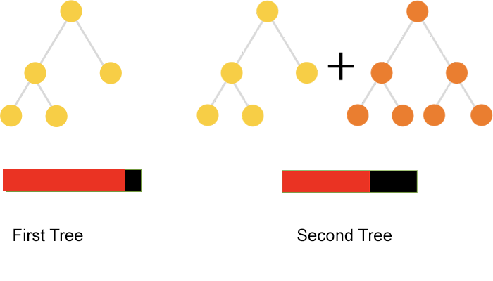
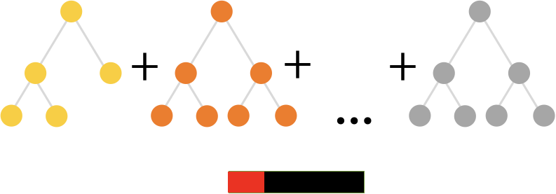
The right-hand image in figure 1 shows the second iteration, in which the algorithm learns one more tree to reduce the error made by the first tree. The algorithm repeats this procedure until it builds a decent quality mode, as we see in figure 2:
Gradient Boosting is a way to implement this idea for any continuous objective function. The common approach for classification uses Logloss while regression optimizes using root mean square error. Ranking tasks commonly implements some variation of LambdaRank.
Each step of Gradient Boosting combines two steps:
- Computing gradients of the loss function we want to optimize for each input object
- Learning the decision tree which predicts gradients of the loss function
The first step is usually a simple operation which can be easily implemented on CPU or GPU. However, the search for the best decision tree is a computationally taxing operation since it takes almost all the time of the GBDT algorithm.
Decision tree learning
Dealing with ordered inputs in GBDT requires fitting decision trees in an iterative manner. Let’s discuss how it is done. For simplicity, we’ll talk about classification trees, which can be easily described.
Classification and regression decision trees are learned in a greedy way. Finding the next tree requires you to calculate all possible feature splits (feature value less than some predefined value) of all the features in the data, then select the one that improves the loss function by the largest value. After the first split is selected, the next split in the tree will be selected in a greedy fashion: the first split is fixed, and the next one is selected given the first one. This operation is repeated until the whole tree is built.
For example, assume we have two input features, user age and music track length, graphed in figure 3, and want to predict whether the user will like the song or not.
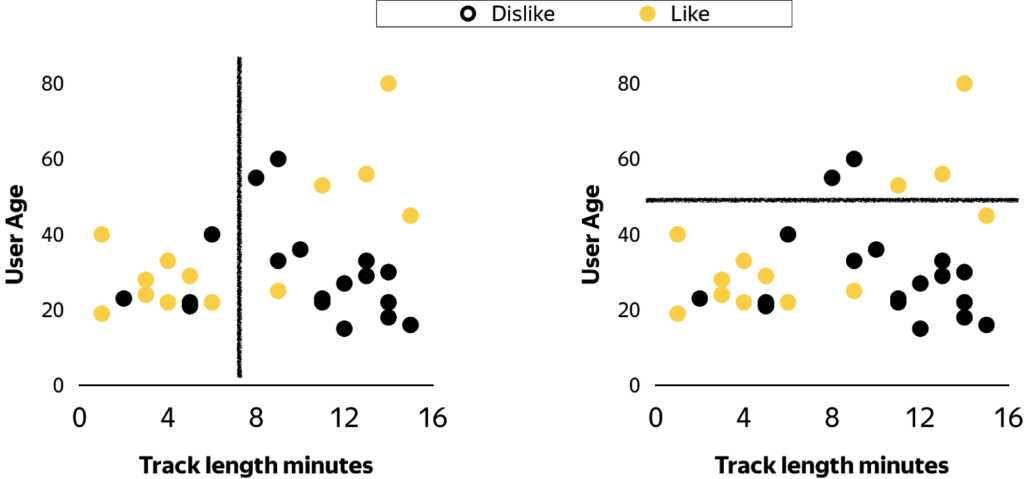
Figure 3. Like / dislike distribution and possible splits
The algorithm evaluates all possible splits of track length and chooses the best one. This is a brute-force approach—we just iterate through all conditions to find the best result. For the problem from the picture we should split the points by music track length, approximately equal to 8 minutes.
Now we have two partitions and the next step is to select one of them to split once again, this time by age. The algorithm repeats, selecting a partition and splitting it by some feature until we reach the stopping condition, shown in figure 4.
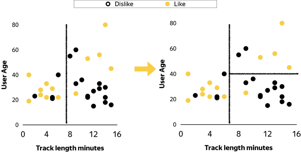
Figure 4. Splitting process
Different stopping conditions and methods of selecting the next partition lead to different learning schemes. The most well-known of these are the leaf-wise and depth-wise approaches.
In the leaf-wise approach, the algorithm splits the partition to achieve the best improvement of the loss function and the procedure continues until we obtain a fixed number of leaves. The algorithm in the depth-wise approach builds the tree level by level until a tree of a fixed depth is built.
CatBoost uses symmetric or oblivious trees. The trees from the music example above are symmetric. In fact, they can be represented as decision tables, as figure 5 shows.
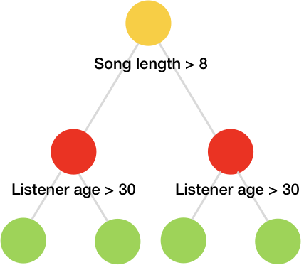
Figure 5. Decision tree for music example
CatBoost uses the same features to split learning instances into the left and the right partitions for each level of the tree. In this case a tree of depth k has exactly 2k leaves, and the index of a leaf can be calculated with simple bitwise operations.
Thus, the CatBoost learning scheme is essentially depth-wise with some simplification, obtained from our decision tree type.
The choice of oblivious trees has several advantages compared to the classic ones:
- Simple fitting scheme
- Efficient to implement on CPU
- Ability to make very fast model appliers
- This tree structure works as a regularization, so it can provide quality benefits for many tasks
Classical decision tree learning algorithm is computation-intensive. To find the next split, we need to evaluate feature count times observation count for different splitting conditions. This leads to a vast number of possible splits for large datasets using continuous inputs and, in many cases, also leads to overfitting.
Fortunately, boosting allows us to significantly reduce the number of splits that we need to consider. We can make a rough approximation for input features. For example, if we have music track length in seconds, then we can round it off to minutes. Such conversions could be done for any ordered features in an automatic way. The simplest way is to use quantiles of input feature distribution to quantize it. This approach is similar in spirit to using 4 or 8 bit floats for neural networks and other compression techniques applied in deep learning.
Thus, boosting each input could be considered as an integer with several distinct values. By default, CatBoost approximates ordered inputs with 7-bit integers (128 different values).
In the next section we’ll discuss how to compute decision trees with 5-bit integers as inputs. These inputs are easier to explain, and we will use them to show the basic idea of computation scheme.
Histograms
If our inputs contain only 5-bit integers, we need to evaluate feature count times 32 different splitting conditions. This quantity does not depend on the number of rows in the input dataset. It also allows us to make an efficient distributed learning algorithm suitable for running on multiple GPUs.
The search for the best split now is just a computation of histograms, shown in figure 6.
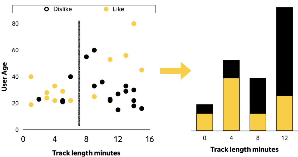
Figure 6. Split now is just a computation of histograms
For each input integer feature, we need to compute the number of likes and dislikes for each feature value for classification or two similar statistics for regression. For decision tree learning we compute two statistics simultaneously, sum of gradients and sum of weights.
We use fast shared memory to make aggregation. Since the size of the shared memory is restricted, we group several features in one to achieve maximum performance gain. If every computation block works with 4 features and 2 statistics simultaneously, we can make an efficient histogram layout and computation pipeline.
The basic idea is simple: allocate an independent histogram per warp. The layout of the histogram should be done in such a way that any operation in shared memory would cause no bank conflicts. So the threads in a warp should work with distinct modulo 32 addresses. The algorithm splits the warp shared memory histogram into four groups. The first eight threads will work with the first histogram group, the second eight threads will do the second group, and so on.
Memory access is done with the following indexing:
32 * bin + 2 * featureId +statisticId + 8 * groupId, where groupId = (threadIdx.x&31)/8
This layout is shown on the figure 7 below.
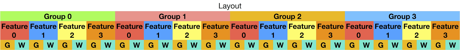
The layout has a nice property: bank conflicts for memory access do not depend on the input data. The data-dependent part of shared memory addresses always gives 0 modulo 32, 32 * bin.
Thus, if 2 * featureId +statisticId + 8 * groupId provide different addresses modulo 32, then we would have shared memory operation without bank conflicts.
This could be achieved if updates in shared memory are done in several passes. On the first pass, the first thread works with the first feature and the first statistic, the second thread works with the first feature and the second statistic, the third thread works with the second feature and the third statistic and so on.
On the second pass each thread works with the other statistic: the first thread works with the first feature and the second statistic, the second thread works with the first feature and the first statistic.
On the third pass the first thread works with the second feature, the third thread works with the third feature and so on. Below you can see the pseudo-code for updating statistics for one point:
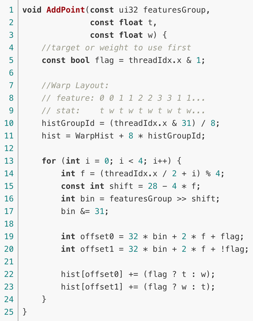
As you can see, the operations hist[offset0] += (flag ? t : w); and hist[offset1] += (flag ? w : t); use distinct modulo 32 addresses, so there is no bank conflicts during aggregation.
This histogram computation scheme makes an important trade-off—no atomic operations in exchange for less occupancy.
Thus, for 32-bin histograms, 2 statistics and 4 features per thread block, we could run at most 384 threads, needing 48KB of shared memory to store shared memory histograms. As a result, our kernel achieves at most 38% of occupancy of Maxwell and later hardware. On Kepler we have just 19% occupancy.
A simple benchmark proves these numbers. First, double the number of working threads in kernel. Now the first 384 threads and second 384 threads are writing to the same addresses with atomic operations, so we have at most two-way atomic conflicts. As you can see from the charts in figure 8 below, the atomic version is slower despite bigger occupancy.
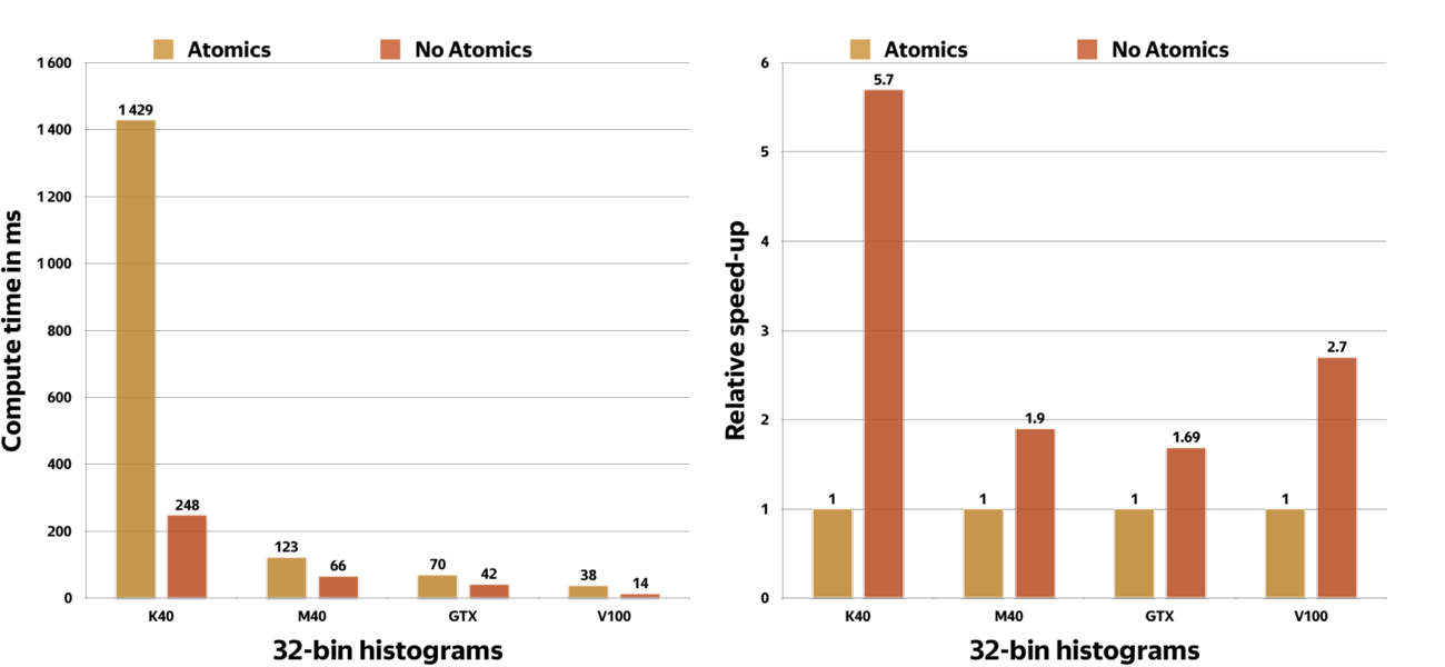
Figure 8. Atomic vs non-atomics 32-bin histograms for different GPU generations
This benchmark measured histogram computation time for the first tree level, the most computationally intensive operation. For deeper levels, fewer gains result from avoiding atomics on Maxwell and newer devices lower because we need to make random access to memory and atomic operations will be hidden by memory latency. However, on deeper levels less computation is required.
We’ve also implemented histograms specializations for 15-bin histograms, 64-bin histograms, 128-bin histograms and 255-bin histograms. Different problems need different numbers of bits to approximate input floats in an optimal way. In some cases 5-bits is enough while others need 8-bits to achieve the best result. CatBoost approximates floats with 7-bit integers by default. Our experiments show this default offers good enough quality. At the same time, this default might be changed for some datasets. If one cares about learning speed, using 5-bits as inputs could give huge benefits in terms of speed while being still generating good quality results.
Categorical features
CatBoost is a special version of GBDT: it perfectly solves problems with ordered features while also supporting categorical features. Categorical feature is a variable that can take one of a limited, and usually fixed number of possible values (categories). For instance, ‘animal’ feature could be set to ‘cat’, ‘dog’, ‘rat’, etc.
Dealing with categorical features efficiently is one of the biggest challenges in machine learning.
The most widely used technique to deal with categorical predictors is one-hot-encoding. The original feature is removed and a new binary variable is added for each category. For example, if the categorical feature was animal, then new binary variables will be added – if this object is a ‘cat’, if this object is a ‘dog’ and so on.
This technique has disadvantages:
- It needs to build deep decision trees to recover dependencies in data in case of features with high cardinality. This can be solved with hashing trick: categorical features are hashed into several different bins (often 32-255 bins are used). However, this approach still significantly affects the resulting quality.
- Doesn’t work for unknown category values, i.e., the values that don’t exist in the learn dataset.
Another way of dealing with categorical features which often provides superior quality compared to hashing and/or one-hot-encoding is to use the so-called label-encoding technique that converts discrete categories to numerical features. Label-encoding can also be used in online-learning systems. We will explain this technique for classification problem below, but it can also be generalized to other tasks.
Since a decision tree works well with numeric inputs we should convert categorical factors to numerical. Let’s replace a categorical feature with several statistics, computed from labels. Assume we have datasets of user/song pairs (u,s)i and labels yi (did the user like the song or not?). For each pair there is a set of features with one feature being a music genre.
We can use categorical feature music genre to estimate probability of the user liking a song:
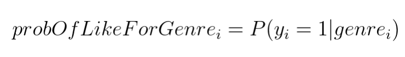
We can use this estimate as a new numerical feature probOfLikeForGenre.
Such probability can be estimated using the learning data in the following way:
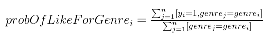
Here [proposition] is represented by an Iverson bracket: value is equal to 1 if the proposition is satisfied, and it is equal to 0 otherwise.
This is a decent approach but could lead to overfitting. For example, if we have a genre that is seen only once in the whole training dataset, then the value of the new numerical feature will be equal to the label value.
In CatBoost we use combination of two following techniques to avoid overfitting:
- Use bayesian estimators with predefined prior
- Estimate probabilities using a scheme, inspired by online-learning
As a result, our estimators have the following form:
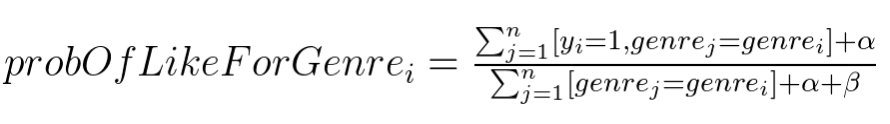
The math behind these formulas is fully explained in two of our papers https://arxiv.org/abs/1706.09516 and http://learningsys.org/nips17/assets/papers/paper_11.pdf.
GPU calculation of the desired statistics is simple. You need to group samples by values of genre using RadixSort. Next, run SegmentedScan primitive to compute numerator and denominator statistics. Finally use Scatter operation to obtain a new feature.
One problem with the proposed solution is that the new features do not account well for feature interactions. For example, user tastes could be very different, and their likes for different genres can be different. One person could like rock and hate jazz, the second could love jazz and hate rock. Sometimes combinations of the features can provide new insights about the data. It is not possible to build all features combinations because there are too many.
We have implemented a greedy algorithm to search for feature combinations to solve this problem and still use combinations. We need to compute success rate estimators on the fly for generated combinations. This can’t be done in the preprocessing stage and need to be accelerated on the GPU.
Now that we have described above the way to compute the numeric statistics, the next step is to efficiently group samples by several features instead of a single feature. We built perfect hashes for feature combinations from source ones to accomplish this. This is done efficiently with standard GPU techniques: RadixSort + Scan + Scatter/Gather.
Performance
The next part of this post contains different comparisons that show performance of the library.
Below we will describe in details when it is efficient to use GPUs instead of CPUs for training. Need to say that comparing different ML frameworks on GPUs is a challenge that is beyond the scope of this post; we refer an interested reader to a recent paper «Why every GBDT speed benchmark is wrong» that goes into related issues in detail.
CPU vs GPU
The first benchmark shows the speed comparison of CPU versus GPU. For this benchmark we have used a dual-socket Intel Xeon E5-2660v4 machine with 56 logical cores and 512GB of RAM as a baseline and several modern GPUs (Kepler K40, Maxwell M40, Pascal GTX 1080Ti and Volta V100) as competitors.
The CPU used in this comparison is very powerful; more mainstream CPUs would show larger differences relative to GPUs.
We couldn’t find a big enough openly available dataset to measure performance gains on GPUs, because we wanted to have a dataset with huge numbers of objects to show how the speedup changes when the dataset grows. So, we’ve used an internal Yandex dataset with approximately 800 ordered features and different sample counts. You can see the results of this benchmark in figure 9.
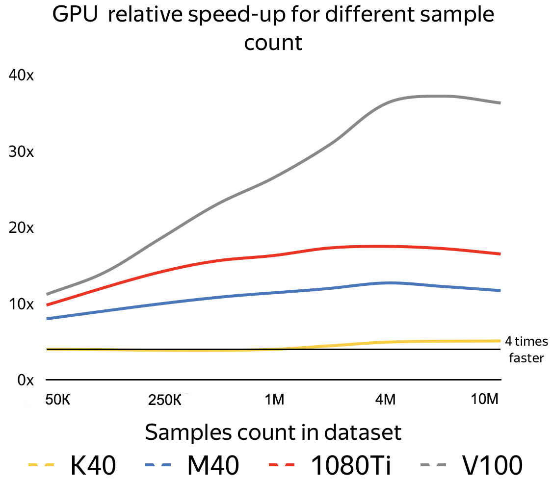
Figure 9. Relative speed-ups of GPUs compared to dual-socket Intel Xeon E5-2660v4 server.
Even a powerful CPU can’t beat a Kepler K40 on large datasets. Volta demonstrates an even more impressive gain, almost 40 times faster than the CPU, without any Volta-specific optimizations.
For multi-classification mode, we see even greater performance gains. Some of our internal datasets which include 200 features, 4659476 objects and 80 classes train on a Titan V 90 to 100 times faster than the CPU.
The main takeaway from this chart: the more data you have, the bigger the speedup. It makes sense to use GPU starting from some tens of thousands of objects. The best results from GPU are observed with big datasets containing several million examples.
Distributed learning
CatBoost can be efficiently trained on several GPUs in one machine. However, some of our datasets at Yandex are too big to fit into 8 GPUs, which is the maximum number of GPUs per server.
NVIDIA announced servers with 16 GPUs with 32GB of memory on each GPU at the 2018 GTC, but dataset sizes become bigger each year, so even 16 GPUs may not be enough. This prompted us to implement the first open source boosting library with computation on distributed GPUs, enabling CatBoost to use multiple hosts for accelerated learning.
Computations scale well over multiple nodes. The chart below shows the training time for the first 200 iteration of some Yandex production formulas in different setups: one machine with onboard GPUs, connected with PCIe, two machines, with 2,4 or 8 GPUs per machine, connected via 1GbE, and two systems with 2,4, or 8 GPUs, connected with Mellanox InfiniBand 56Gb.
CatBoost achieves good scalability as shown in the chart in figure 10. On 16 GPUs with InfiniBand, CatBoost runs approximately 3.75 faster than on 4 GPUs. The scalability should be even better with larger datasets. If there is enough data, we can train models on slow 1GbE networks, as two machines with two cards per machine are not significantly slower than 4 GPUs on one PCIe root complex.
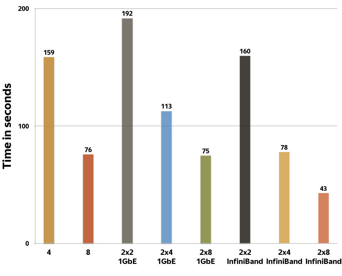
Figure 10. CatBoost scalability for multi-GPU learning with different GPU interconnections (PCI, 1GbE, Mellanox InfiniBand)
Conclusion
In this post we have described the CatBoost algorithm and basic ideas we’ve used to build its GPU version. Our GPU library is highly efficient and we hope that it will provide great benefits for our users. It is very easy to start using GPU training with CatBoost and you can train models using Python, R or, command line binary, which you can review in our documentation. Give it a try!
This is a repost of CatBoost team member, Vasily Ershov, article from nVidia developer blog .